5  ParlGov losers’ consent

Losers’ consent models example – see also sections “Party-voted-for in government” and “Performance of Party Facts linking” in manuscript.

library(conflicted)

library(tidyverse)
conflicts_prefer(dplyr::filter, .quiet = TRUE)
library(glue)
library(knitr)

library(broom) # tidy model results
library(broom.mixed) # tidy model results for lme4
library(estimatr) # robust standard errors
library(ggeffects) # effects plots
library(lme4) # multi-level models
library(modelsummary) # model tables and coefficient plots
library(patchwork) # combine plots
library(reactable) # dynamic tables
library(skimr) # summary statistics

options(knitr.kable.NA = "")

round_numeric_variables <- function(data, digits = 0) {
  mutate(data, across(
    where(is.numeric),
    \(.x) format(round(.x, digits), scientific = FALSE)
  ))
}

ess_raw <- read_rds("data/02-ess-select.rds")
ess_cabinet_raw <- read_rds("data/07-parlgov-ess_cabinets.rds")

5.1 Losers’ consent models

Satisfaction with democracy by those that voted for parties in government vs. opposition. For a book length discussion and empirical assessment of European democracies see Anderson et.al. (2005) – esp. model page 104. A replication and extension to other regions is provided by Farrer and Zingher (2019, 525)

• Anderson, Christopher, ed. 2005. Losers’ Consent: Elections and Democratic Legitimacy. Oxford ; New York: Oxford University Press.
• Farrer, Benjamin, and Joshua N Zingher. 2019. “A Global Analysis of How Losing an Election Affects Voter Satisfaction with Democracy.” International Political Science Review 40(4): 518–34. — doi: 10.1093/poq/nfad003

5.2 Variables

Variables used in losers’ consent models and context information

• stfdem — How satisfied with the way democracy works in country?
  • 0 // Extremely dissatisfied — 10 // Extremely satisfied
• cabinet — “party-voted-for” (prtv) in government after election
  • ParlGov based calculation
  • excluding caretaker governments
• lrscale — Placement on left right scale
  • 0 // Left — 10 // Right
• gndr — Gender
• agea — Age of respondent, calculated
• eduyrs — Years of full-time education completed
• ESS identifiers
  • cntry — Country
  • essround — ESS round
  • pspwght — Post-stratification weight // see ESS survey weights
  • inw_date — Date of interview // various ESS inw* variables
• Party information
  • prtv — Party voted for in last national election // aggregated ESS IDs
  • prtv_name — Party voted for in last national election // party name
  • first_ess_id — unique ESS party ID used in Party Facts

5.3 Summary statistics

ess_cabinet <-
  ess_cabinet_raw |>
  select(essround, cntry, idno, cabinet = cabinet_party)

ess_lm <-
  ess_raw |>
  left_join(ess_cabinet) |>
  mutate(
    across(c(lrscale, stfdem), \(.x) as.integer(.x) - 1),
    cabinet = case_when(
      cabinet == 1 ~ "Yes",
      cabinet == 0 ~ "No",
      .default = NA
    ),
    cabinet = as.factor(cabinet) |> fct_rev()
  ) |>
  filter(!all(is.na(cabinet)), .by = c(cntry, essround))

ess_lm |>
  select(-idno) |>
  skim() |>
  round_numeric_variables(2)

Data summary

Name	select(ess_lm, -idno)
Number of rows	433599
Number of columns	14
_______________________
Column type frequency:
character	3
Date	1
factor	4
numeric	6
________________________
Group variables	None

Variable type: character

skim_variable	n_missing	complete_rate	min	max	empty	n_unique	whitespace
cntry	0	1.00	2	2	0	32	0
prtv	171780	0.60	8	14	0	2704	0
prtc	240202	0.45	8	10	0	2642	0

Variable type: Date

skim_variable	n_missing	complete_rate	min	max	median	n_unique
inw_date	912	1.00	2002-01-14	2022-09-02	2011-06-03	4827

Variable type: factor

skim_variable	n_missing	complete_rate	ordered	n_unique	top_counts
gndr	331	1.00	FALSE	2	Fem: 231527, Mal: 201741, No : 0
prtv_party	171780	0.60	FALSE	888	Lab: 6580, Con: 6077, Chr: 5660, Soc: 4972
prtc_party	240202	0.45	FALSE	900	Lab: 4949, Con: 4578, Chr: 4290, Soc: 3484
cabinet	209243	0.52	FALSE	2	Yes: 121092, No: 103264

Variable type: numeric

skim_variable	n_missing	complete_rate	mean	sd	p0	p25	p50	p75	p100	hist
essround	0	1.00	5.39	2.80	1	3.0	5.00	8.00	10.00	▇▇▇▇▇
pspwght	0	1.00	1.01	0.52	0	0.7	0.93	1.18	6.85	▇▁▁▁▁
agea	2155	1.00	48.49	18.62	13	33.0	48.00	63.00	123.00	▆▇▆▁▁
eduyrs	5075	0.99	12.43	4.13	0	10.0	12.00	15.00	65.00	▇▅▁▁▁
lrscale	55413	0.87	5.13	2.23	0	4.0	5.00	7.00	10.00	▂▃▇▃▁
stfdem	15516	0.96	5.28	2.51	0	4.0	5.00	7.00	10.00	▅▅▇▇▂

5.4 Multi-level models (ML)

Model variables preparation

• removing outliers age (99% quantile)
• selecting only variables used in models
• removing incomplete observations
• centering of continuous variables (age, education, left-right)

# quantile(ess_lm$eduyrs, probs = c(0, 0.5, 0.9, 0.95, 0.99, 0.999), na.rm = TRUE)
eduyrs_remove <- quantile(ess_lm$eduyrs, probs = 0.99, na.rm = TRUE)

ess_lm_c <-
  ess_lm |>
  filter(eduyrs < eduyrs_remove) |>
  select(stfdem, cabinet, gndr, eduyrs, agea, lrscale, cntry, essround, pspwght) |>
  na.omit() |>
  mutate(
    essround_cntry = paste(essround, cntry),
    across(c(agea, eduyrs, lrscale),
      \(.x) scale(.x, scale = FALSE) |> as.vector(),
      .names = "{.col}_c"
    )
  )

plot_ggpredict <- function(model, plot_terms) {
  ggpredict(model, terms = plot_terms) |>
    plot(show.title = FALSE, show.legend = FALSE)
}

ml_formula <- "stfdem ~ gndr +  cabinet*eduyrs_c + cabinet*poly(agea_c, 2) + cabinet*poly(lrscale_c, 2)"

5.4.1 Three ML models

Multi-level models with quadric terms and interactions. Structure of models:

• Model 1 (ML-1) — ESS-Round/country and country
• Model 2 (ML-2) — ESS-Round and country
• Model 3 (ML-3) — country

Visualization of results in Figure 5.1 and Figure 5.2 – see variable information in Section 5.3

ml1 <- lmer(
  as.formula(glue("{ml_formula} + (1 | cntry/essround_cntry)")),
  weights = pspwght,
  data = ess_lm_c
)

ml2 <- lmer(
  as.formula(glue("{ml_formula} + (1 | essround) + (1 | cntry)")),
  weights = pspwght,
  data = ess_lm_c
)

ml3 <- lmer(
  as.formula(glue("{ml_formula} + (1 | cntry)")),
  weights = pspwght,
  data = ess_lm_c
)

models <- list("ML-1" = ml1, "ML-2" = ml2, "ML-3" = ml3)

if (knitr::is_html_output()) {
  modelsummary(models)
} else {
  modelsummary(models, output = "markdown")
}

	ML-1	ML-2	ML-3
(Intercept)	5.785	5.793	5.778
	(0.168)	(0.183)	(0.171)
gndrFemale	−0.182	−0.178	−0.179
	(0.009)	(0.010)	(0.010)
cabinetNo	−0.637	−0.644	−0.639
	(0.010)	(0.010)	(0.010)
eduyrs_c	0.048	0.045	0.048
	(0.002)	(0.002)	(0.002)
poly(agea_c, 2)1	23.619	21.026	25.707
	(3.151)	(3.193)	(3.189)
poly(agea_c, 2)2	30.466	30.402	31.450
	(2.914)	(2.958)	(2.968)
poly(lrscale_c, 2)1	103.655	105.276	108.504
	(3.334)	(3.204)	(3.209)
poly(lrscale_c, 2)2	35.915	39.317	40.238
	(3.117)	(3.149)	(3.161)
cabinetNo × eduyrs_c	0.013	0.014	0.015
	(0.003)	(0.003)	(0.003)
cabinetNo × poly(agea_c, 2)1	−4.492	−2.175	−3.764
	(4.619)	(4.674)	(4.691)
cabinetNo × poly(agea_c, 2)2	13.570	14.312	14.018
	(4.284)	(4.350)	(4.366)
cabinetNo × poly(lrscale_c, 2)1	−21.845	−23.387	−26.187
	(4.861)	(4.493)	(4.496)
cabinetNo × poly(lrscale_c, 2)2	−108.662	−113.510	−113.724
	(4.367)	(4.397)	(4.413)
SD (Intercept cntry)	0.926	0.959	0.964
SD (Observations)	2.106	2.142	2.150
SD (Intercept essround_cntrycntry)	0.502
SD (Intercept essround)		0.219
Num.Obs.	205661	205661	205661
R2 Marg.	0.040	0.040	0.041
R2 Cond.	0.232	0.207	0.202
AIC	918475.2	924653.1	926121.1
BIC	918639.0	924816.9	926274.6
ICC	0.2	0.2	0.2
RMSE	2.13	2.16	2.17

Analysis of variance (ANOVA) models and refitting with Maximum Likelihood instead of Restricted Maximum Likelihood.

anova(ml1, ml2, ml3) |>
  tidy() |>
  arrange(term)

term	npar	AIC	BIC	logLik	deviance	statistic	df	p.value
ml1	16	918470.1	918633.8	-459219.0	918438.1	7648.019	1	0
ml2	16	924648.2	924811.9	-462308.1	924616.2	0.000	0
ml3	15	926116.1	926269.6	-463043.0	926086.1

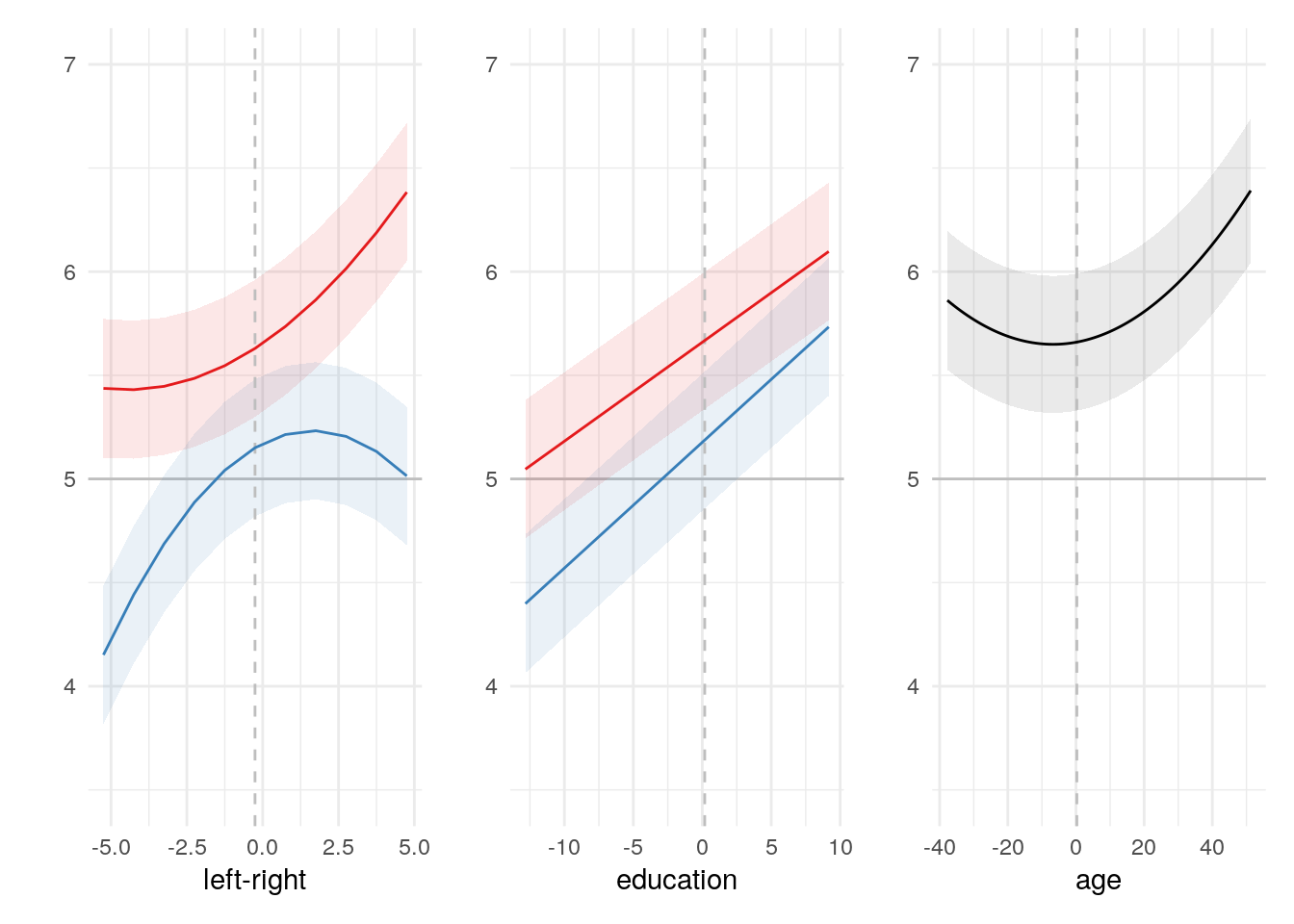
5.4.2 Effects plot ML-1

Effects plot Multi-Level Model 1 (ML-1, see Section 5.4.1)

plot_ggpredict(ml1, c("lrscale_c [all]", "cabinet")) +
  plot_ggpredict(ml1, c("agea_c [all]", "cabinet")) +
  plot_ggpredict(ml1, c("eduyrs_c [all]", "cabinet"))

Figure 5.1: Effects plot (95% CIs) — Satisfaction with democracy

pl_dt_lr <- ggpredict(ml1, c("lrscale_c [all]", "cabinet"))
pl_dt_edu <- ggpredict(ml1, c("eduyrs_c [all]", "cabinet"))
pl_dt_age <- ggpredict(ml1, c("agea_c [all]"))

add_plot_layers <- function(pl, var_name = "x") {
  pl +
    geom_hline(yintercept = 5, color = "grey", size = 0.5) +
    geom_ribbon(aes(ymin = conf.low, ymax = conf.high), alpha = 0.1) +
    scale_y_continuous(limits = c(3.5, 7)) +
    labs(x = var_name, y = "") +
    theme_minimal()
}

color_values <- c("Yes" = "#E41A1C", "No" = "#377EB8")

pl_lr <-
  ggplot(pl_dt_lr, aes(x, predicted, fill = group)) |>
  add_plot_layers("left-right") +
  geom_vline(xintercept = median(ess_lm_c$lrscale_c), color = "grey", size = 0.5, linetype = "dashed") +
  geom_line(aes(colour = group)) +
  guides(color = "none", fill = "none") +
  scale_color_manual(values = color_values) +
  scale_fill_manual(values = color_values)

pl_edu <-
  ggplot(pl_dt_edu, aes(x, predicted, fill = group)) |>
  add_plot_layers("education") +
  geom_vline(xintercept = median(ess_lm_c$eduyrs_c), color = "grey", size = 0.5, linetype = "dashed") +
  geom_line(aes(colour = group)) +
  guides(color = "none", fill = "none") +
  scale_color_manual(values = color_values) +
  scale_fill_manual(values = color_values)

pl_age <-
  ggplot(pl_dt_age, aes(x, predicted)) |>
  add_plot_layers("age") +
  geom_vline(xintercept = median(ess_lm_c$agea_c), color = "grey", size = 0.5, linetype = "dashed") +
  geom_line()

pl <- pl_lr + pl_edu + pl_age

ggsave("figures-tables/figure-2_ml-model-effects.png", pl, width = 9, height = 6, dpi = 300)
pl

Figure 5.2: Effects plot (95% CIs) — Satisfaction with democracy // Article version

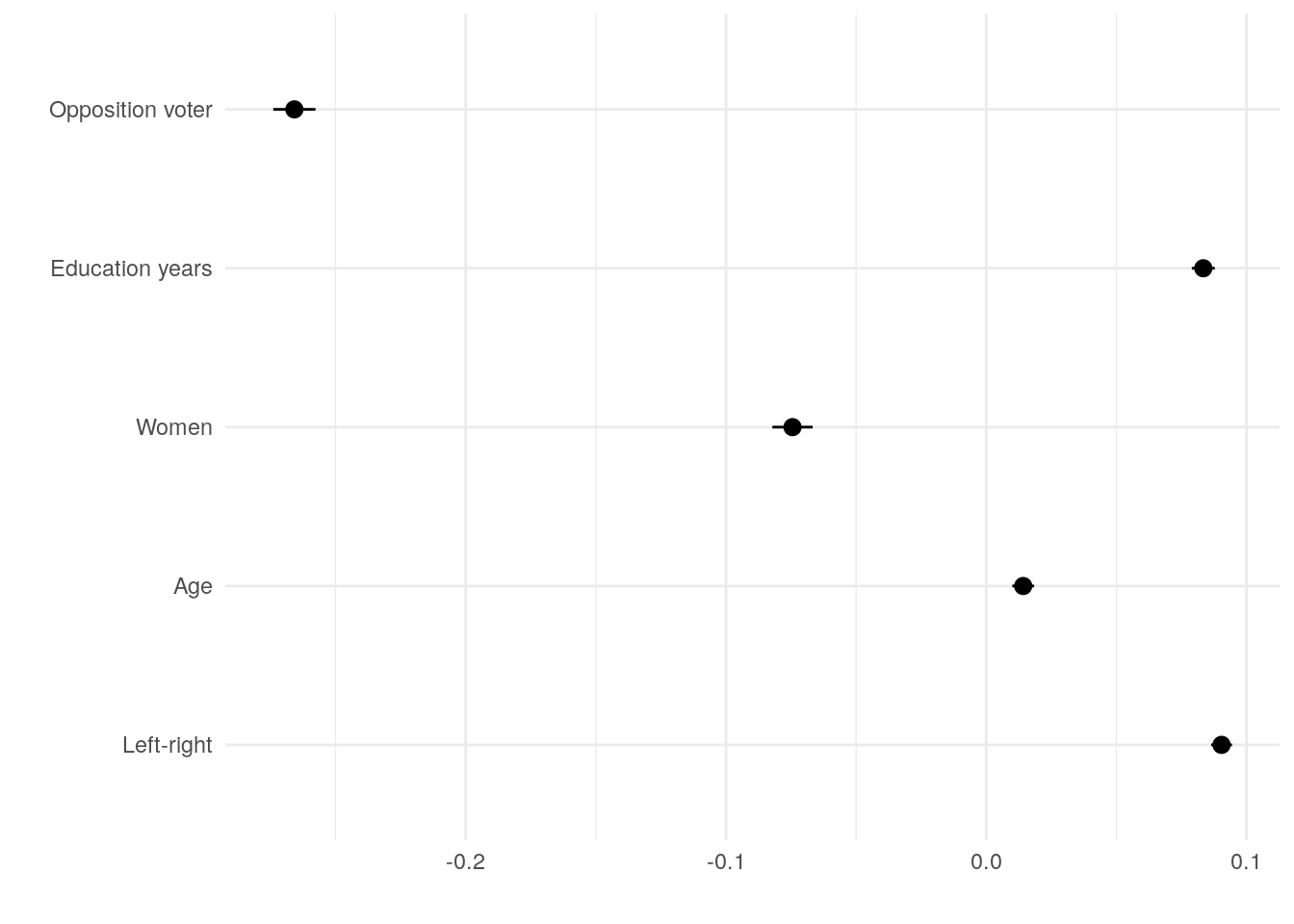
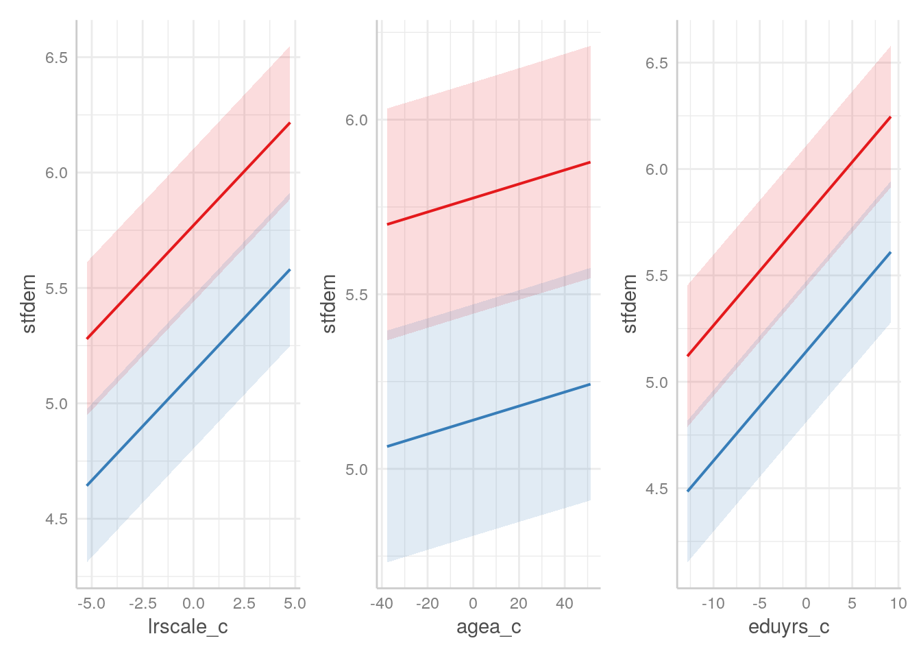
5.5 Linear effects (ML)

Multi-level model with linear terms and no interactions.

Visualization of results in Figure 5.3 (standardized coefficients) and Figure 5.4 (effects) – see variable information in Section 5.3

ml_le <- lmer(
  "stfdem ~ cabinet + gndr + eduyrs_c + agea_c + lrscale_c + (1 | cntry/essround_cntry)",
  weights = pspwght,
  data = ess_lm_c
)

ml_le |>
  tidy() |>
  kable(digits = 3)

effect	group	term	estimate	std.error	statistic
fixed		(Intercept)	5.778	0.169	34.171
fixed		cabinetNo	-0.636	0.010	-64.301
fixed		gndrFemale	-0.178	0.009	-18.843
fixed		eduyrs_c	0.051	0.001	37.008
fixed		agea_c	0.002	0.000	6.639
fixed		lrscale_c	0.094	0.002	44.202
ran_pars	essround_cntry:cntry	sd__(Intercept)	0.505
ran_pars	cntry	sd__(Intercept)	0.930
ran_pars	Residual	sd__Observation	2.111

cm <- c(
  "cabinetNo" = "Opposition voter",
  "eduyrs_c" = "Education years",
  "gndrFemale" = "Women",
  "agea_c" = "Age",
  "lrscale_c" = "Left-right"
)

# parameters::parameters(ml1, standardize = "refit")
# modelplot(ml_le)

modelplot(ml_le, coef_map = rev(cm), standardize = "refit") +
  labs(x = "")

Figure 5.3: Standardized coefficients (95% CIs)– Linear effects model

plot_ggpredict(ml_le, c("lrscale_c [all]", "cabinet")) +
  plot_ggpredict(ml_le, c("agea_c [all]", "cabinet")) +
  plot_ggpredict(ml_le, c("eduyrs_c [all]", "cabinet"))

Figure 5.4: Linear effects plot (95% CIs) — Satisfaction with democracy

5.6 Fixed effects model

Fixed effects model with quadric terms and interactions.

Visualization of results in Figure 5.5 and variable information in Section 5.3

m_fe <-
  lm_robust(as.formula(glue("{ml_formula} + cntry + factor(essround)")),
    weights = pspwght,
    data = ess_lm_c
  )

m_fe |>
  tidy() |>
  mutate(
    term = str_remove_all(term, "poly\\(|, 2\\)1"),
    term = str_replace(term, fixed(", 2)2"), "^2")
  ) |>
  filter(!str_starts(term, "cntry|factor")) |>
  select(-df, -outcome) |>
  kable(digits = 3)

term	estimate	std.error	statistic	p.value	conf.low	conf.high
(Intercept)	6.406	0.037	173.695	0.000	6.334	6.478
gndrFemale	-0.178	0.011	-16.563	0.000	-0.199	-0.157
cabinetNo	-0.644	0.011	-58.760	0.000	-0.666	-0.623
eduyrs_c	0.045	0.002	21.577	0.000	0.041	0.050
agea_c	20.954	3.506	5.977	0.000	14.083	27.825
agea_c^2	30.380	3.306	9.189	0.000	23.900	36.861
lrscale_c	105.286	3.903	26.974	0.000	97.635	112.936
lrscale_c^2	39.358	4.134	9.520	0.000	31.255	47.462
cabinetNo:eduyrs_c	0.014	0.003	4.740	0.000	0.008	0.020
cabinetNo:agea_c	-2.142	5.236	-0.409	0.682	-12.405	8.120
cabinetNo:agea_c^2	14.323	4.958	2.889	0.004	4.606	24.041
cabinetNo:lrscale_c	-23.390	5.585	-4.188	0.000	-34.336	-12.444
cabinetNo:lrscale_c^2	-113.526	5.823	-19.496	0.000	-124.940	-102.113

Fixed effects for countries (“cnty”) and ESS rounds (“essround”) not shown.

m_fe |>
  glance() |>
  kable(digits = 2)

r.squared	adj.r.squared	statistic	p.value	df.residual	nobs	se_type
0.18	0.18	755.96	0	205608	205661	HC2

plot_ggpredict(m_fe, c("lrscale_c [all]", "cabinet")) +
  plot_ggpredict(m_fe, c("agea_c [all]", "cabinet")) +
  plot_ggpredict(m_fe, c("eduyrs_c [all]", "cabinet"))

Figure 5.5: Fixed effects model (95% CIs) — Satisfaction with democracy

5.7 Share covered

id_select <- "parlgov_id" # "ches_id" + "parlgov_id"
ess_check <- ess_cabinet_raw # ess_raw + ess_cabinet_raw
tbl_file_name <- "figures-tables/table-2b_parlgov-coverage.csv"

We calculate the share of matches for the “party-voted-for” (prtv) question. Excluded from the calculation are instances of other, independent, and technical (see Party Facts codebook).

link_table_technical <-
  read_rds("data/03-party-facts-links-technical.rds")

prtv <-
  ess_check |>
  left_join(link_table_technical, by = c("prtv" = "ess_id")) |>
  select(cntry, essround, prtv, prtv_party, all_of(id_select), partyfacts_name, technical) |>
  filter(!is.na(prtv)) |>
  mutate(is_match = if_else(is.na(.data[[id_select]]), 0, 1))

prtv_match <-
  prtv |>
  filter(technical != 7 & technical != 8 & technical != 12 | is.na(technical)) |>
  summarise(
    prvt_n = n(),
    is_match = first(is_match),
    .by = c(cntry, essround, prtv, prtv_party)
  )

prtv_share <-
  prtv_match |>
  summarise(
    share_match = (sum(prvt_n * is_match) * 100 / sum(prvt_n)) |> round(1),
    .by = c(cntry, essround)
  )

The table summarizes the share of party matches across all countries and ESS rounds.

tbl_out <-
  prtv_share |>
  reframe(
    enframe(
      quantile(share_match, c(0, 0.1, 0.25, 0.5, 0.75, 1)),
      "quantile", "share_match"
    )
  ) |>
  mutate(share_match = round(share_match, 1))

write_csv(tbl_out, tbl_file_name)
tbl_out

quantile	share_match
0%	11.4
10%	65.4
25%	81.9
50%	95.8
75%	99.2
100%	100.0

The share of matched parties is weighted by the number of “party-voted-for” responses and is calculated for each country in every ESS round.

The next table summarizes the country level share of party matches for ESS rounds with data set matches.

tbl_out <-
  prtv_share |>
  summarise(
    min = min(share_match),
    median = median(share_match) |> round(1),
    max = max(share_match),
    ess_rounds = n_distinct(essround),
    .by = cntry
  ) |>
  filter(max > 0) |>
  arrange(min, median)

if (knitr::is_html_output()) {
  tbl_out |>
    reactable(searchable = TRUE, striped = TRUE)
} else {
  tbl_out
}