4 CHES left-right validation

ESS linking example – see also sections “Expert survey validation” and “Performance of Party Facts linking” in manuscript.

Code

library(conflicted)

library(tidyverse)
conflicts_prefer(dplyr::filter, .quiet = TRUE)
library(glue)
library(knitr)

library(ggforce) # violin plots
library(reactable)

Code

ches_raw <- haven::read_dta("data-raw/ches-1999-2019_CHES_dataset_meansv3-td4m.dta")
ess_raw <- read_rds("data/05-ess-ches.rds")
ess_all_raw <- read_rds("data/02-ess-select.rds")

4.1 CHES information

Chapel Hill Expert Survey (CHES) series

Code

ches_raw |>
  summarise(
    countries = n_distinct(country),
    parties = n(),
    .by = year
  )

year	countries	parties
1999	14	142
2002	23	171
2006	24	188
2010	24	203
2014	28	245
2019	28	247

4.2 CHES and ESS

Number of countries and parties that are included in ESS and CHES for an ESS round.

Code

ess_raw |>
  summarize(
    year = first(year),
    countries_n = n_distinct(cntry),
    parties_n = n_distinct(prtv),
    ches_year = first(ches_year),
    ches_parties_n = n_distinct(ches_id),
    .by = c(essround)
  ) |>
  arrange(essround)

essround	year	countries_n	parties_n	ches_year	ches_parties_n
1	2002	18	196	2002	131
2	2004	18	190	2002	128
3	2006	18	191	2006	132
4	2008	21	215	2006	143
5	2010	20	241	2010	157
6	2012	20	239	2010	151
7	2014	18	216	2014	138
8	2016	18	216	2014	133
9	2018	24	299	2014	184
10	2020	23	284	2019	169

Overview country coverage ESS and CHES trend file

ess_cntry — number of countries in ESS round
ches_cntry — number of ESS round countries in CHES
ches_missing — names of ESS round countries not in CHES

Code

cntry_ches_n <-
  ess_raw |>
  summarise(ches_cntry = n_distinct(cntry), .by = essround)

cntry_ches_none <-
  ess_all_raw |>
  distinct(essround, cntry) |>
  anti_join(distinct(ess_raw, essround, cntry)) |>
  arrange(cntry) |>
  summarise(ches_missing = paste0(cntry, collapse = ", "), .by = essround)

ess_all_raw |>
  summarise(ess_cntry = n_distinct(cntry), .by = essround) |>
  left_join(cntry_ches_n) |>
  left_join(cntry_ches_none) |>
  arrange(essround)

essround	ess_cntry	ches_cntry	ches_missing
1	22	18	CH, IL, LU, NO
2	25	18	CH, EE, IS, LU, NO, TR, UA
3	23	18	CH, CY, NO, RU, UA
4	29	21	CH, CY, HR, IL, NO, RU, TR, UA
5	27	20	CH, CY, HR, IL, NO, RU, UA
6	29	20	AL, CH, CY, IL, IS, NO, RU, UA, XK
7	21	18	CH, IL, NO
8	23	18	CH, IL, IS, NO, RU
9	29	24	CH, IS, ME, NO, RS
10	30	23	CH, IL, IS, ME, MK, NO, RS

4.3 Country-year correlation

Code

ess_party <-
  ess_raw |>
  filter(!is.na(prtv)) |>
  summarise(
    lr_mean = mean(lrscale, na.rm = TRUE),
    lr_sd = sd(lrscale, na.rm = TRUE),
    lr_n = n(),
    ches_lr = first(ches_lr),
    .by = c(cntry, year, prtv, prtv_party, ches_year),
  )

Country-year correlations for ESS and CHES left-right positions in each ESS round with at least 3 parties and 10 responses per party in a country.

ESS left-right party positions are calculated as mean values of lrscale variables for respondents that voted for the party (prtv*).

lrscale — self-placement on left right scale // ESS rounds
prtv* — “party-voted-for” in last national election // ESS rounds
ches_lr — left-right party position // CHES trend file
- lrgen — “position of the party in YEAR in terms of its overall ideological stance.” // CHES trendfile

Code

ess_party_filter <-
  ess_party |>
  na.omit() |>
  filter(lr_n >= 10) |>
  mutate(n = n(), .by = c(cntry, year)) |>
  filter(n >= 3)

corr <-
  ess_party_filter |>
  summarise(
    n_parties = first(n),
    lr_corr = cor(lr_mean, ches_lr, use = "pairwise.complete.obs"),
    .by = c(cntry, year, ches_year)
  ) |>
  arrange(cntry, year)

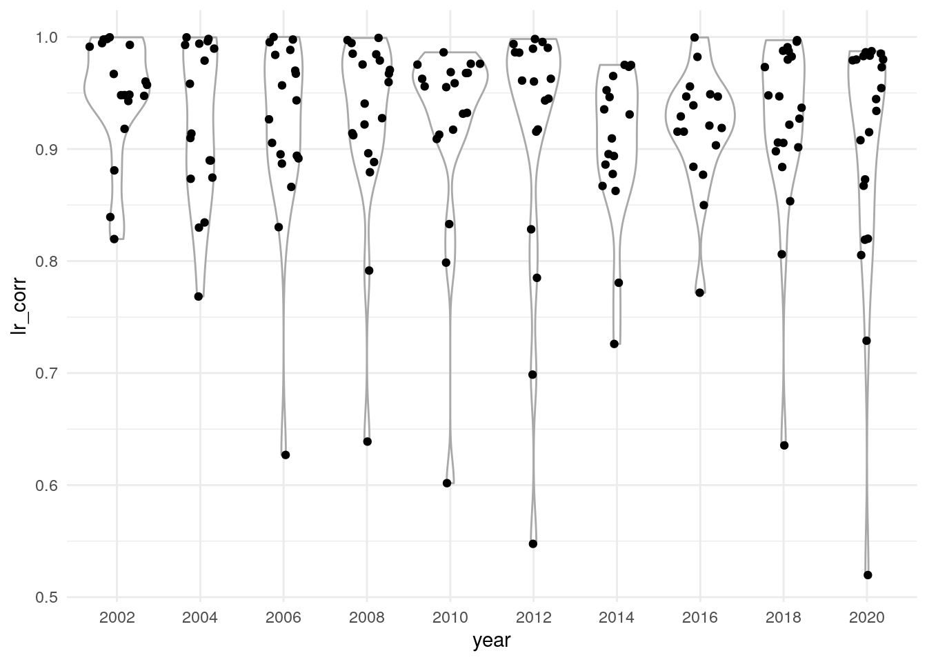
# fivenum(corr$lr_corr)

The table summarizes the country-year correlations by providing 0%, 10%, 25%, 50%, 75%, and 100% quantiles. The results are visualized in Figure 4.1.

Code

tbl_out <-
  corr |>
  summarise(
    p0 = quantile(lr_corr, 0),
    p10 = quantile(lr_corr, 0.10),
    p25 = quantile(lr_corr, 0.25),
    p50 = quantile(lr_corr, 0.50),
    p75 = quantile(lr_corr, 0.75),
    p100 = quantile(lr_corr, 1),
    .by = year
  ) |>
  mutate(across(p0:p100, \(x) round(x, 2))) |>
  rename(ess_year = year) |>
  arrange(ess_year)

write_csv(tbl_out, "figures-tables/table-3_ches-validation.csv")
tbl_out

ess_year	p0	p10	p25	p50	p75	p100
2002	0.82	0.87	0.94	0.95	0.99	1.00
2004	0.77	0.83	0.87	0.91	0.99	1.00
2006	0.63	0.86	0.89	0.93	0.98	1.00
2008	-0.35	0.79	0.90	0.94	0.98	1.00
2010	0.45	0.78	0.91	0.96	0.97	0.99
2012	0.55	0.76	0.92	0.96	0.99	1.00
2014	0.73	0.83	0.88	0.91	0.95	0.98
2016	0.77	0.87	0.90	0.92	0.95	1.00
2018	0.26	0.81	0.90	0.93	0.98	1.00
2020	0.35	0.56	0.82	0.93	0.98	0.99

Country-year correlations by country // interactive table

Code

if (knitr::is_html_output()) {
  corr |>
    mutate(lr_corr = round(lr_corr, 2)) |>
    reactable(searchable = TRUE, striped = TRUE)
}

Code

ro_2008 <-
  ess_party |>
  filter(lr_n >= 10) |>
  filter(cntry == "RO", year == 2008) |>
  left_join(distinct(ess_raw, prtv, prtv_party)) |>
  mutate(lr_mean = round(lr_mean, 2)) |>
  select(-lr_sd)

ro_2008_cor <-
  cor(ro_2008$lr_mean, ro_2008$ches_lr, use = "pairwise.complete.obs") |>
  round(2)

Lowest country-year correlation (-0.35) for ESS Romania 2008.

Code

ro_2008 |>
  arrange(prtv) |>
  select(cntry, year, prtv, prtv_party, lr_n, lr_mean, ches_year, ches_lr)

cntry	year	prtv	prtv_party	lr_n	lr_mean	ches_year	ches_lr
RO	2008	RO-4-1-v	PD-L	517	6.95	2006	NA
RO	2008	RO-4-12-v	Other: PIN	14	5.25	2006	NA
RO	2008	RO-4-2-v	Alianta PSD-PC	449	3.52	2006	NA
RO	2008	RO-4-3-v	PNL	165	7.06	2006	6.7
RO	2008	RO-4-4-v	PRM	31	4.54	2006	7.0
RO	2008	RO-4-5-v	UDMR	67	5.94	2006	6.0
RO	2008	RO-4-6-v	PNG-CD	15	6.75	2006	NA
RO	2008	RO-4-9-v	PNTCD	32	5.62	2006	NA

Code

corr |>
  filter(lr_corr >= 0.5) |>
  mutate(year = factor(year)) |>
  ggplot(aes(year, lr_corr)) +
  geom_violin(colour = "darkgrey") +
  geom_sina() +
  theme_minimal()

Figure 4.1: Violin plot for country wise correlations ( < 0.5 removed)

4.4 Share covered

Code

id_select <- "ches_id" # "ches_id" + "parlgov_id"
ess_check <- ess_raw # ess_raw + ess_cabinet_raw
tbl_file_name <- "figures-tables/table-2a_ches-coverage.csv"

We calculate the share of matches for the “party-voted-for” (prtv) question. Excluded from the calculation are instances of other, independent, and technical (see Party Facts codebook).

Code

link_table_technical <-
  read_rds("data/03-party-facts-links-technical.rds")

prtv <-
  ess_check |>
  left_join(link_table_technical, by = c("prtv" = "ess_id")) |>
  select(cntry, essround, prtv, prtv_party, all_of(id_select), partyfacts_name, technical) |>
  filter(!is.na(prtv)) |>
  mutate(is_match = if_else(is.na(.data[[id_select]]), 0, 1))

prtv_match <-
  prtv |>
  filter(technical != 7 & technical != 8 & technical != 12 | is.na(technical)) |>
  summarise(
    prvt_n = n(),
    is_match = first(is_match),
    .by = c(cntry, essround, prtv, prtv_party)
  )

prtv_share <-
  prtv_match |>
  summarise(
    share_match = (sum(prvt_n * is_match) * 100 / sum(prvt_n)) |> round(1),
    .by = c(cntry, essround)
  )

The table summarizes the share of party matches across all countries and ESS rounds.

Code

tbl_out <-
  prtv_share |>
  reframe(
    enframe(
      quantile(share_match, c(0, 0.1, 0.25, 0.5, 0.75, 1)),
      "quantile", "share_match"
    )
  ) |>
  mutate(share_match = round(share_match, 1))

write_csv(tbl_out, tbl_file_name)
tbl_out

quantile	share_match
0%	11.4
10%	54.6
25%	87.7
50%	98.4
75%	99.9
100%	100.0

The share of matched parties is weighted by the number of “party-voted-for” responses and is calculated for each country in every ESS round.

The next table summarizes the country level share of party matches for ESS rounds with data set matches.

Code

tbl_out <-
  prtv_share |>
  summarise(
    min = min(share_match),
    median = median(share_match) |> round(1),
    max = max(share_match),
    ess_rounds = n_distinct(essround),
    .by = cntry
  ) |>
  filter(max > 0) |>
  arrange(min, median)

if (knitr::is_html_output()) {
  tbl_out |>
    reactable(searchable = TRUE, striped = TRUE)
} else {
  tbl_out
}