Public broadcasting Germany

Today, there was a decision about a public broadcasting reform in Germany.

There were suggestions to reduce the number of public broadcasters before the meeting of the Minister-presidents.

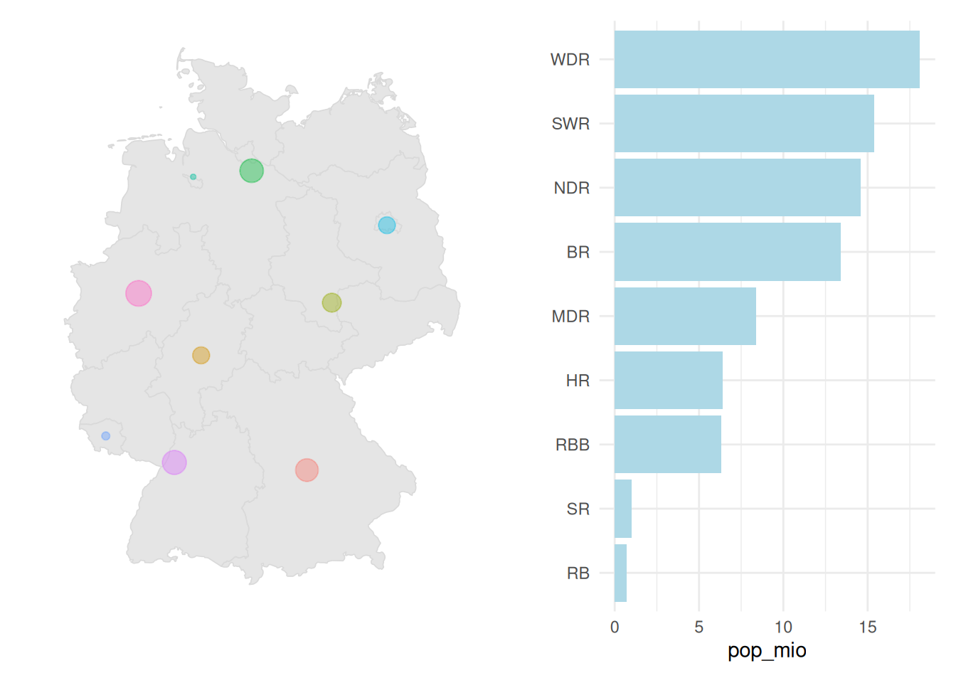
So, I was interested in the state’s population, which is covered by German public broadcasters.

Code

library(conflicted) # create errors for function name conflicts

library(tidyverse)
conflicts_prefer(dplyr::filter, .quiet = TRUE)

library(sf)
library(patchwork)

ggplot2::theme_set(theme_minimal())

Code

states_raw <- read_csv("rundfunk-laender.csv")
map_raw <- read_rds("r-ne_states-deu.rds")

## Broadcaster ----

services <-
  map_raw |>
  inner_join(states_raw) |>
  summarise(
    n = n(),
    pop_sum = sum(population),
    pop_mio = NA,
    states = paste0(sort(state), collapse = ", "),
    geometry = st_union(geometry) |> st_centroid(),
    .by = service
  ) |>
  mutate(pop_mio = round(pop_sum / 1e6, 1)) |>
  select(-pop_sum) |>
  arrange(service)

Code

pl_dt <-
  services |>
  mutate(service = fct_reorder(factor(service), pop_mio))

## bar chart
pl1 <-
  ggplot(pl_dt, aes(x = pop_mio, y = service)) +
  geom_col(fill = "lightblue") +
  labs(y = "")

# map German states
pl2 <-
  ggplot() +
  geom_sf(data = map_raw, colour = "grey85", lwd = 0.3) +
  geom_sf(data = services, aes(size = pop_mio, colour = service), alpha = 0.4) +
  coord_sf(crs = "EPSG:4839") + # LCC projection Germany
  guides(colour = "none", size = "none") +
  theme_void()

pl2 + pl1 + plot_layout(widths = c(3, 2))

Code

ggsave("broadcaster-deu.png", pl2, width = 3, height = 5, dpi = 300)

services |>
  st_drop_geometry()

service	n	pop_mio	states
BR	1	13.4	BY
HR	1	6.4	HE
MDR	3	8.4	SN, ST, TH
NDR	4	14.6	HH, MV, NI, SH
RB	1	0.7	HB
RBB	2	6.3	BB, BE
SR	1	1.0	SL
SWR	2	15.4	BW, RP
WDR	1	18.1	NW

Sources

Statistische Ämter des Bundes und der Länder, dl-de/by-2-0
- Fläche und Bevölkerung nach Ländern
Natural Earth